EKF SLAM 调参小记
Basic Algorithm
\[
\mu = \begin{pmatrix} x & y & \theta & m_{1,x} & m_{1,y} & m_{2,x} & m_{2,y} & \cdots & m_{n,x} & m_{n,y} \end{pmatrix}^T
\in \mathbf{R}^{2N+3}
\]
\[
\Sigma=\begin{pmatrix}
\sigma_{xx} & \sigma_{xy} & \sigma_{x\theta} & \sigma_{xm_{1,x}} & \sigma_{xm_{1,y}} & \cdots & \sigma_{xm_{n,x}} & \sigma_{xm_{n,y}} \\
\sigma_{yx} & \sigma_{yy} & \sigma_{y\theta} & \sigma_{ym_{1,x}} & \sigma_{ym_{1,y}} & \cdots & \sigma_{ym_{n,x}} & \sigma_{ym_{n,y}} \\
\sigma_{\theta x} & \sigma_{\theta y} & \sigma_{\theta \theta} & \sigma_{\theta m_{1,x}} & \sigma_{\theta m_{1,y}} & \cdots & \sigma_{\theta m_{n,x}} & \sigma_{\theta m_{n,y}} \\
\sigma_{m_{1,x}x} & \sigma_{m_{1,x}y} & \sigma_{m_{1,x}\theta} & \sigma_{m_{1,x}m_{1,x}} & \sigma_{m_{1,x}m_{1,y}} & \cdots & \sigma_{m_{1,x}m_{n,x}} & \sigma_{m_{1,x}m_{n,y}} \\
\sigma_{m_{1,y}x} & \sigma_{m_{1,y}y} & \sigma_{m_{1,y}\theta} & \sigma_{m_{1,y}m_{1,x}} & \sigma_{m_{1,y}m_{1,y}} & \cdots & \sigma_{m_{1,y}m_{n,x}} & \sigma_{m_{1,y}m_{n,y}} \\
\vdots &\vdots &\vdots &\vdots &\vdots &\ddots &\vdots &\vdots \\
\sigma_{m_{n,x}x} & \sigma_{m_{n,x}y} & \sigma_{m_{n,x}\theta} & \sigma_{m_{n,x}m_{1,x}} & \sigma_{m_{n,x}m_{1,y}} & \cdots & \sigma_{m_{n,x}m_{n,x}} & \sigma_{m_{n,x}m_{n,y}} \\
\sigma_{m_{n,y}x} & \sigma_{m_{n,y}y} & \sigma_{m_{n,y}\theta} & \sigma_{m_{n,y}m_{1,x}} & \sigma_{m_{n,y}m_{1,y}} & \cdots & \sigma_{m_{n,y}m_{n,x}} & \sigma_{m_{n,y}m_{n,y}} \\
\end{pmatrix}
\in \mathbf{R}^{(2N+3)\times(2N+3)}
\]
Prediction
For certain control input \(u_t=\begin{pmatrix}v_t\\\omega_t\end{pmatrix}\) , we have \(\bar{\mu_t}=g(u_t,\mu_{t-1})\), which is
\[
\bar{\mu_t}=
\begin{pmatrix}
\bar{x_t} \\ \bar{y_t} \\ \bar{\theta_t} \\ \vdots
\end{pmatrix}
=
\begin{pmatrix}
x_{t-1} \\ y_{t-1} \\ \theta_{t-1} \\ \vdots
\end{pmatrix}
+
\begin{pmatrix}
\frac{v_t}{\omega_t}(-\sin\theta_{t-1}+\sin(\theta_{t-1}+\omega_t\Delta t)) \\
\frac{v_t}{\omega_t}(+\cos\theta_{t-1}-\cos(\theta_{t-1}+\omega_t\Delta t)) \\
\omega_t\Delta t \\
\bf0
\end{pmatrix}
\]
Then \(\bar{\Sigma_t}=G_t\Sigma_{t-1}G_t^T+B_tQ_tB_t^T\), which \(G_t\) and \(B_t\) is the jacobian matrix, \(Q_t\) is the covariance of your noise
\[
\begin{aligned}
G_t &= \frac{\partial g(u_t,\mu_{t-1})}{\partial\mu} \\
&= \frac{\partial}{\partial\mu}
\left[
\begin{pmatrix}
x_{t-1} \\ y_{t-1} \\ \theta_{t-1} \\ \vdots
\end{pmatrix}
+
\begin{pmatrix}
\frac{v_t}{\omega_t}(-\sin\theta_{t-1}+\sin(\theta_{t-1}+\omega_t\Delta t)) \\
\frac{v_t}{\omega_t}(+\cos\theta_{t-1}-\cos(\theta_{t-1}+\omega_t\Delta t)) \\
\omega_t\Delta t \\
\bf0
\end{pmatrix}
\right]
\\
&=I+\frac{\partial}{\partial\mu}
\begin{pmatrix}
\frac{v_t}{\omega_t}(-\sin\theta_{t-1}+\sin(\theta_{t-1}+\omega_t\Delta t)) \\
\frac{v_t}{\omega_t}(+\cos\theta_{t-1}-\cos(\theta_{t-1}+\omega_t\Delta t)) \\
\omega_t\Delta t \\
\bf0
\end{pmatrix} \\
&=I+
\begin{pmatrix}
0&0&\frac{v_t}{\omega_t}(-\cos\theta_{t-1}+\cos(\theta_{t-1}+\omega_t\Delta t))&0&\cdots&0 \\
0&0&\frac{v_t}{\omega_t}(-\sin\theta_{t-1}+\sin(\theta_{t-1}+\omega_t\Delta t))&0&\cdots&0 \\
0&0&0&0&\cdots&0\\
0&0&0&0&\cdots&0\\
\vdots&\vdots&\vdots&\vdots&\ddots&\vdots \\
0&0&0&0&\cdots&0\\
\end{pmatrix} \\
&=
\begin{pmatrix}
1&0&\frac{v_t}{\omega_t}(-\cos\theta_{t-1}+\cos(\theta_{t-1}+\omega_t\Delta t))&0&\cdots&0 \\
0&1&\frac{v_t}{\omega_t}(-\sin\theta_{t-1}+\sin(\theta_{t-1}+\omega_t\Delta t))&0&\cdots&0 \\
0&0&1&0&\cdots&0\\
0&0&0&1&\cdots&0\\
\vdots&\vdots&\vdots&\vdots&\ddots&\vdots \\
0&0&0&0&\cdots&1\\
\end{pmatrix} \in \mathbf{R}^{(2N+3)\times(2N+3)}
\end{aligned}
\]
\[
B_t=
\begin{pmatrix}
\frac{+\sin(\theta_{t-1}+\omega_t\Delta t)-\sin\theta_{t-1}}{\omega_t}
&
\frac{v_t\left[-\sin(\theta_{t-1}+\omega_t\Delta t)+\sin\theta_{t-1}\right]}{\omega_t^2} + \frac{v_t\Delta t\cos(\theta_{t-1}+\omega_t\Delta t)}{\omega_t}
\\
\frac{-\cos(\theta_{t-1}+\omega_t\Delta t)+\cos\theta_{t-1}}{\omega_t}
&
\frac{v_t\left[+\cos(\theta_{t-1}+\omega_t\Delta t)-\cos\theta_{t-1}\right]}{\omega_t^2} - \frac{v_t\Delta t\sin(\theta_{t-1}+\omega_t\Delta t)}{\omega_t}
\\
0&\Delta t\\
0&0\\
\vdots&\vdots\\
0&0
\end{pmatrix}\in \mathbf{R}^{(2N+3)\times2}
\]
Update
For a certain observed feature i, if there is a certain landmark j, whose coordinate is \(\bar\mu_j=\begin{pmatrix}\mu_{j,x}\\\mu_{j,y}\end{pmatrix}\) in the world axis , is corresponding to expected to i. We can model it's observation result by range and bearing.
\[
\delta=\begin{pmatrix}\delta_x\\\delta_y\end{pmatrix}=\begin{pmatrix}\bar\mu_{j,x}-\bar\mu_{t,x}\\\bar\mu_{j,y}-\bar\mu_{t,y}\end{pmatrix}
\]
\[
h(\bar\mu_t)=\hat z_t^j = \begin{pmatrix}||\delta||_2\\\arctan(\delta_y/\delta_x)-\bar\mu_{t,\theta}\end{pmatrix}
\]
Do the partial of \(h(\bar\mu_t)\), we can get jacobian matrix \(H_t^j\)
\[
\begin{aligned}
H_t^j&=\frac{\partial h(\bar\mu_t)}{\partial\bar\mu_t}\\&=\frac{\partial}{\partial\bar\mu_t}\begin{pmatrix}||\delta||_2\\\arctan(\delta_y/\delta_x)-\bar\mu_{t,\theta}\end{pmatrix}\\
&=\begin{pmatrix}
-\frac{\delta_x}{||\delta||_2} & -\frac{\delta_y}{||\delta||_2} & 0 & 0 & \cdots & 0 & +\frac{\delta_x}{||\delta||_2} & +\frac{\delta_y}{||\delta||_2} & 0 &\cdots & 0 \\
+\frac{\delta_y}{||\delta||_2^2} & -\frac{\delta_x}{||\delta||_2^2} & -1 & 0 & \cdots & 0 & -\frac{\delta_y}{||\delta||_2^2} & +\frac{\delta_x}{||\delta||_2^2} & 0 &\cdots &0
\end{pmatrix}\in \mathbf R^{2\times(2N+3)}
\end{aligned}
\]
The \(3+(2j-2)+1\)-th column and the \(3+(2j-2)+2\)-th column correspond to the j-th landmark
\(R_t\) is the noise of the sensor, then the kalman gain could be calculated
\[
K_t^j=\bar\Sigma_tH_t^{jT}(H_t^j\bar\Sigma_tH_t^{jT}+R_t)^{-1}
\]
And then update the estimation and the covariance of the pose for all landmarks iteratively
\[
\bar\mu_t = \bar\mu_t+K_t^j(z_t^j-\hat z_t^j)
\]
\[
\bar\Sigma_t=(I-K_t^jH_t^j)\bar\Sigma_t
\]
If the feature have never seen before, we just simply expand our feature vector and the covariance matrix to contain it.
Attempts
Alpha
The mathematical descriptions were mainly given above, but there are still two missing parameters \(Q_t\) and \(R_t\). They are the covariance matrix of the noise of control input \(u_t\) and the observation model \(z_t\).
For the observation model, we use Kalman Gain to determine whether the sensor can be trust or not.
\[
K_t^j=\bar\Sigma_tH_t^{jT}(H_t^j\bar\Sigma_tH_t^{jT}+R_t)^{-1}
\]
When \(R_t=0\), \(K_t^j=\bar\Sigma_tH_t^{jT}(H_t^j\bar\Sigma_tH_t^{jT}+R_t)^{-1}=(H_t^j)^{-1}\) which means we have a perfect sensor is noise free.
When \(R_t\to\infty\), \(K_t^j=\bar\Sigma_tH_t^{jT}(H_t^j\bar\Sigma_tH_t^{jT}+R_t)^{-1}\to0\) which means we won't believe the result of the horrible sensor.
In lab's case, I pick \(R_t=\begin{pmatrix}1.0*10^{-2} & 0 \\ 0 & 1.0*10^{-3}\end{pmatrix}\), which gave me a good performance.
Although we don't have a gain or some other things to describe the affect of noise in control input model explicitly, the affect of the \(Q_t\) to the control input is also intuitively. It would some case decrease the belief of the variable, leads to approximating a slightly different gaussian model. I suppose the control input noise is not so significantly to the system. I randomly pick up 100 as the value of the diagnols, which is \(Q_t=\begin{pmatrix}100 & 0 \\ 0 & 100\end{pmatrix}\)
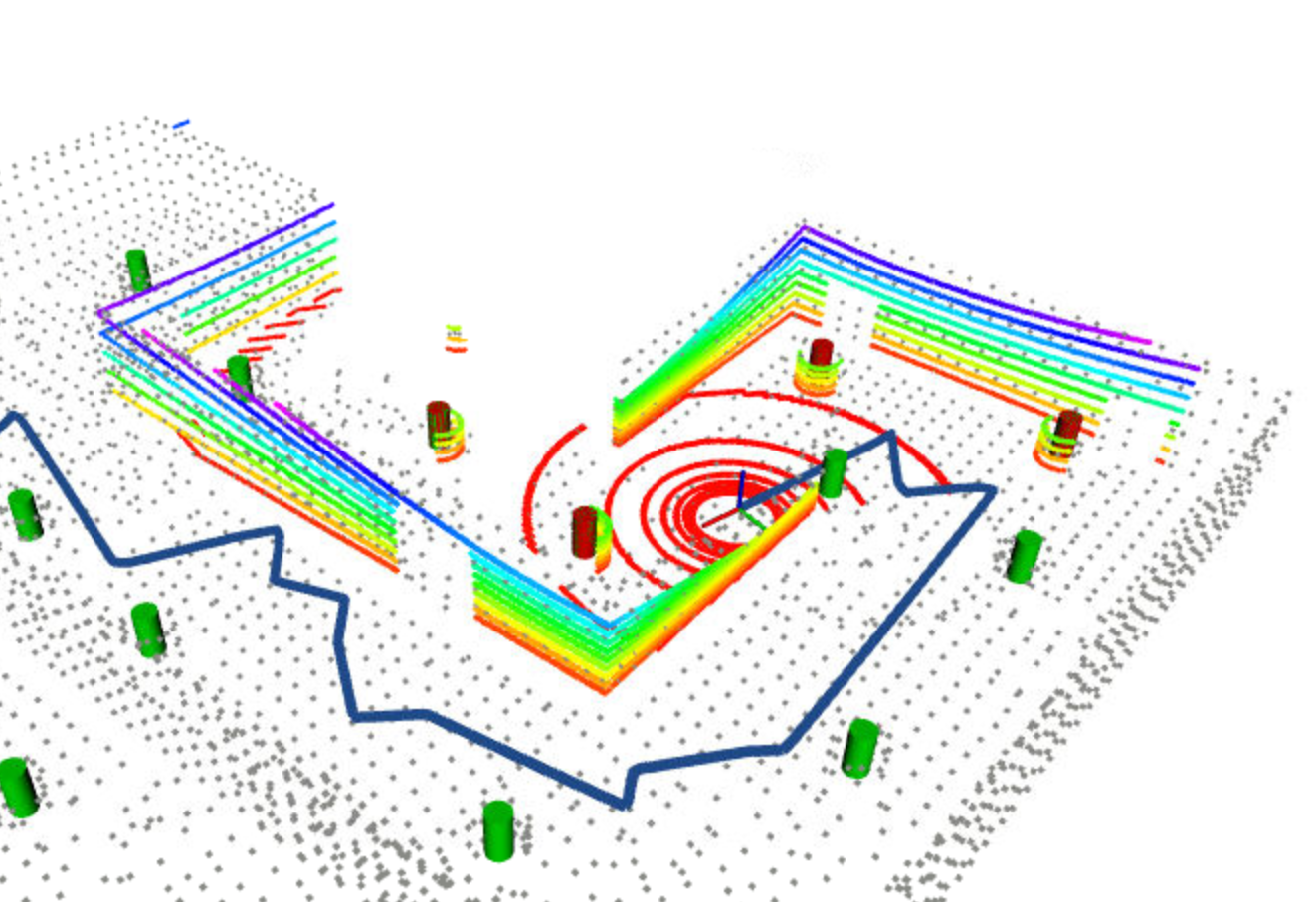
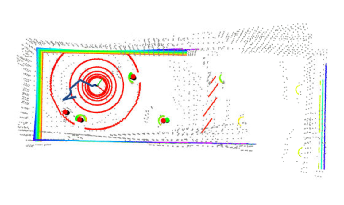
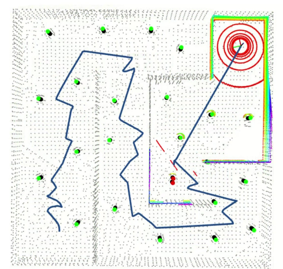
As image shown above, an improper noise covariance matrix may lead to a little bit mess.
Beta
As we all know, EKF SLAM build the correspondence for the closest pair of feature and landmark. Hence, we need to find a proper threshold to distinguish whether the feature is a new landmark or not. A too large threshold will make the system insensitive to establishing new landmarks, while a too small threshold will make the system too sensitive to establishing new landmarks. A good way to get the proper threshold is printing out the distance matrix, and then find that specific value to classify the distance into two groups. That's how I do so, and I eventually pick 4.0
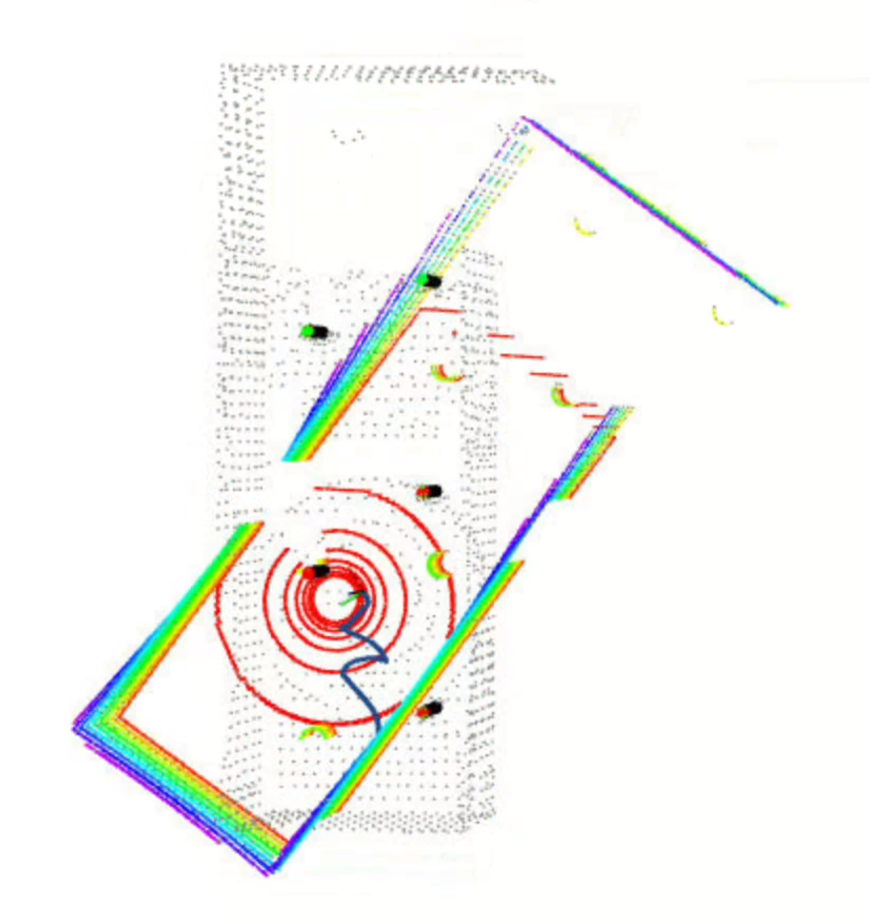
Above image shows the case that new landmarks were not be recognized well, because of a too big threshold, which two new landmarks correspond to a same already-known landmark, leading the EKF SLAM goes wrong in this case. But then it actually worked, although there are some vibrations in that specific case until it gets to another special location.
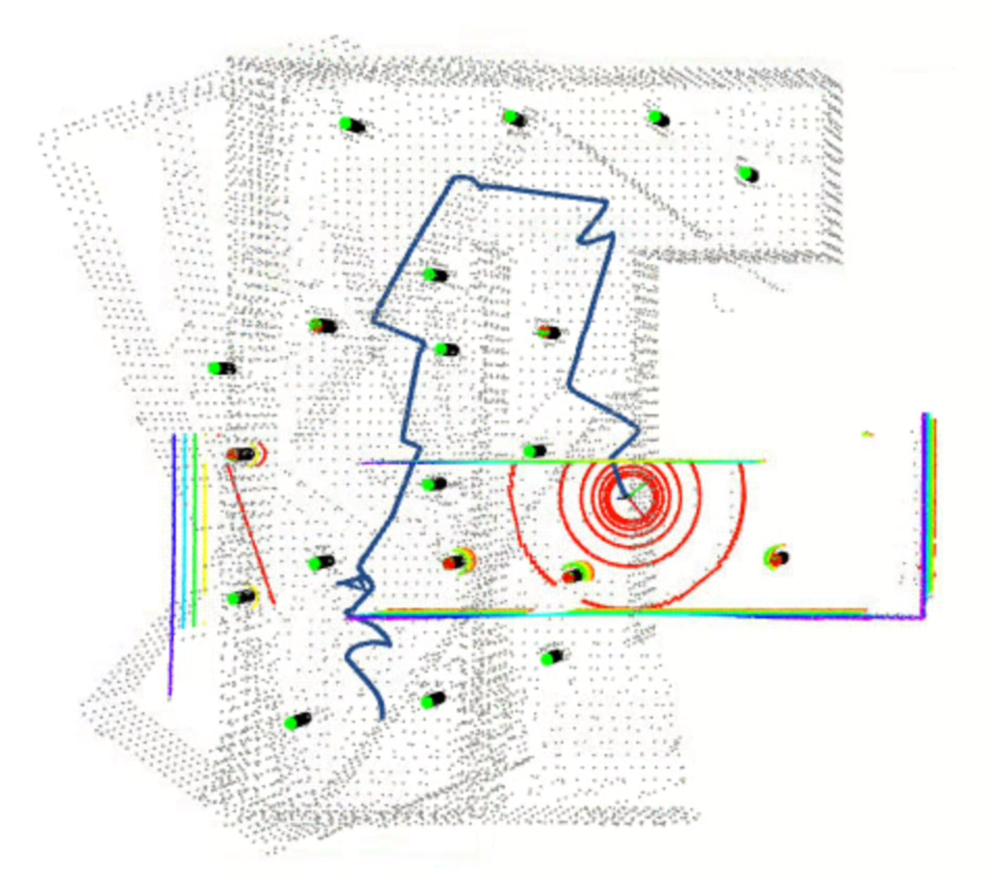
In this special location, because of the previous vibration, some landmarks were wrongly attended to the state vector and the covariance matrix. Next time the robot matches the observed features and landmarks, there is a new feature's distance to the wrong-existing landmark lower than the threshold. Hence, the filter corresponds to them as a pair rather than adding a new landmark to the system, which leads to not converging. This is also what we don't expect from the steady filter. So we need to adjust the threshold smarter.
Gamma
Finally it works, with \(R_t=\begin{pmatrix}1.0*10^{-2} & 0 \\ 0 & 1.0*10^{-3}\end{pmatrix}\), \(Q_t=\begin{pmatrix}100 & 0 \\ 0 & 100\end{pmatrix}\), and \(\delta_{d}=4.0\)
