Detailed derivation of On-Manifold IMU Preintegration

• C. Forster, L. Carlone, F. Dellaert, and D. Scaramuzza, “On-Manifold Preintegration for Real-Time Visual--Inertial Odometry,” IEEE Trans. Robot., vol. 33, no. 1, pp. 1–21, Feb. 2017, doi: 10.1109/TRO.2016.2597321.

• Z. Yang and S. Shen, “Monocular Visual–Inertial State Estimation With Online Initialization and Camera–IMU Extrinsic Calibration,” IEEE Trans. Automat. Sci. Eng., vol. 14, no. 1, pp. 39–51, Jan. 2017, doi: 10.1109/TASE.2016.2550621.

Inertial Measurement Unit (IMU) preintegration is a fundamental technique in visual-inertial odometry that efficiently combines high-frequency IMU measurements between keyframes. This approach, pioneered by Forster et al. and Yang et al., formulates the integration process on the manifold of rigid body motions $SE(3)$, addressing the nonlinear nature of 3D rotations through Lie group theory.

The key innovation lies in separating the integration of IMU measurements from the global state, enabling computationally efficient optimization by precomputing relative motion constraints. This derivation details the mathematical foundations, including the special orthogonal group $SO(3)$, perturbation models, uncertainty representation on manifolds, and the complete preintegration theory that handles sensor biases and noise characteristics while maintaining real-time performance. The resulting preintegrated terms serve as constraints in factor graph optimization frameworks for robust state estimation.

Special Orthology Group $SO(3)$

The special orthology group $SO(3)$ is defined as the set of all ${\mathbb{R}}^{3\times 3}$ rotation matrix:

$$SO(3)=\{R\in {\mathbb{R}}^{3\times 3}:R^{T}R=I,det(R)=1\}$$

And its tagent space on the manifold $\mathfrak{so}(3)$, consist of skew-symmetric matrices:

$$\begin{array}{}\text{(1)}& {\mathit{\omega }}^{\wedge }={\left[\begin{array}{c}{\omega }_1\\ {\omega }_2\\ {\omega }_3\end{array}\right]}^{\wedge }=\left[\begin{array}{ccc}0& -{\omega }_3& {\omega }_2\\ {\omega }_3& 0& -{\omega }_1\\ -{\omega }_2& {\omega }_1& 0\end{array}\right]\in \mathfrak{so}(3)\end{array}$$

The hat operator $(\cdot {)}^{\wedge }$ maps a vector $\mathit{\omega }\in {\mathbb{R}}^3$ to $\mathfrak{so}(3)$, while the vee operator $(\cdot {)}^{\vee }$ performs the inverse mapping.

Rodrigues' Rotation Formula

Let $\mathbf{v}\in {\mathbb{R}}^{\mathbf{3}}$ be a 3D vector to be rotated by a unit vector axis $\mathbf{n}\mathbf{=}\left(\begin{array}{c}{n}_x\\ n_y\\ n_z\end{array}\right)$ by an angle $\theta$. The resulting rotated vector is denoted ${\mathbf{v}}_{\text{rot}}$.

$\mathbf{v}$ can be decomposed to two orthogonal components: the parallel to $\mathbf{n}$ part ${\mathbf{v}}_{\parallel }$ and the perpendicular to $\mathbf{n}$ part ${\mathbf{v}}_{\perp }$. Which satisfy,

$$\{\begin{array}{l}{\mathbf{v}}_{\parallel }=(\mathbf{v}\cdot \mathbf{n})\mathbf{n}\\ {\mathbf{v}}_{\perp }=\mathbf{v}-(\mathbf{v}\cdot \mathbf{n})\mathbf{n}=-\mathbf{n}\times (\mathbf{n}\times \mathbf{v})\end{array}$$

The whole vector $\mathbf{v}$ is then rotated by:

$$\begin{array}{rl}{\mathbf{v}}_{\text{rot}}& ={\mathbf{v}}_{\parallel \text{rot}}+{\mathbf{v}}_{\perp \text{rot}}\\ & ={\mathbf{v}}_{\parallel }+\cos \theta {\mathbf{v}}_{\perp }+\sin \theta \mathbf{n}\times {\mathbf{v}}_{\perp }\\ & =(\mathbf{v}\cdot \mathbf{n})n+\cos \theta {\mathbf{v}}_{\perp }+\sin \theta \mathbf{n}\times \mathbf{v}\\ & =\cos \theta \mathbf{v}+(1-\cos \theta )(\mathbf{n}\cdot \mathbf{v})\mathbf{n}+\sin \theta \mathbf{n}\times \mathbf{v}\end{array}$$

We get Rodrigues' Rotation Formula. Write it on the manifold, we then have:

$$R=\cos (||\varphi ||)I+[1-\cos (||\varphi ||)]\frac{\varphi {\varphi }^T}{||\varphi |{|}^2}+\sin (||\varphi ||){\varphi }^{\wedge }$$

The exponential map $\exp :\mathfrak{so}(3)\to SO(3)$ converts a skew-symmetric matrix into a rotation matrix via the Rodrigues rotation formula:

$$\begin{array}{}\text{(3)}& R=\exp ({\mathit{\varphi }}^{\wedge })=I+\frac{\sin \parallel \mathit{\varphi }\parallel }{\parallel \mathit{\varphi }\parallel }{\mathit{\varphi }}^{\wedge }+\frac{1-\cos \parallel \mathit{\varphi }\parallel }{\parallel \mathit{\varphi }{\parallel }^2}({\mathit{\varphi }}^{\wedge }{)}^2\end{array}$$

For small angles, this simplifies to $R\approx I+{\mathit{\varphi }}^{\wedge }$.

Exponential Mapping

$$\begin{array}{rl}R& =\exp ({\varphi }^{\wedge })\\ & =\sum _{n=0}^{\mathrm{\infty }}\frac{({\varphi }^{\wedge }{)}^n}{n!}\\ & =I+(||\varphi ||-\frac{||\varphi |{|}^3}{3!}+\frac{||\varphi |{|}^5}{5!}+\cdots ){\varphi }^{\wedge }+(\frac{||\varphi |{|}^2}{2!}-\frac{||\varphi |{|}^4}{4!}+\frac{||\varphi |{|}^6}{6!}-\cdots )({\varphi }^{\wedge }{)}^2\\ & =I+\frac{\sin ||\varphi ||}{||\varphi ||}{\varphi }^{\wedge }+\frac{1-\cos ||\varphi ||}{||\varphi |{|}^2}({\varphi }^{\wedge }{)}^2\end{array}$$

The logarithmic map $ \log : SO(3) \to \mathfrak{so}(3) $ extracts the axis-angle representation from a rotation matrix:

$$\begin{array}{}\text{(5)}& \mathit{\varphi }=\log (R{)}^{\vee }=\frac{\parallel \mathit{\varphi }\parallel }{2\sin \parallel \mathit{\varphi }\parallel }\left[\begin{array}{c}{r}_{32}-r_{23}\\ r_{13}-r_{31}\\ r_{21}-r_{12}\end{array}\right]\end{array}$$

Logarithmic Mapping

$$R=I+\frac{\sin ||\varphi ||}{||\varphi ||}{\varphi }^{\wedge }+\frac{1-\cos ||\varphi ||}{||\varphi |{|}^2}({\varphi }^{\wedge }{)}^2$$

So the trace of the rotation matrix satisfied:

$$\begin{array}{rl}\mathrm{t}\mathrm{r}(R)& =\mathrm{t}\mathrm{r}(I)+\frac{\sin ||\varphi ||}{||\varphi ||}\mathrm{t}\mathrm{r}({\varphi }^{\wedge })+\frac{1-\cos ||\varphi ||}{||\varphi |{|}^2}\mathrm{t}\mathrm{r}[({\varphi }^{\wedge }{)}^2]\\ & =3+0+\frac{1-\cos ||\varphi ||}{||\varphi |{|}^2}(-||{\varphi }^{\wedge }|{|}^2)\\ & =3+0+\frac{1-\cos ||\varphi ||}{||\varphi |{|}^2}(-2||\varphi |{|}^2)\\ & =3+2\cos ||\varphi ||-2\end{array}$$

The angle $\theta$ is calculated by

$$||\varphi ||=\arccos (\frac{\mathrm{t}\mathrm{r}(R)-1}{2})+2k\pi$$

When $\varphi \ne 0\iff R\ne I$, we construct a skew part and a non-skew part.

$$R=\underset{\frac{1}{2}(R-R^T)}{\underbrace{\frac{\sin ||\varphi ||}{||\varphi ||}{\varphi }^{\wedge }}}+\underset{\frac{1}{2}(R+R^T)}{\underbrace{I+\frac{1-\cos ||\varphi ||}{||\varphi |{|}^2}({\varphi }^{\wedge }{)}^2}}$$

So

$$\begin{array}{}\text{(5)}& \begin{array}{rl}\varphi & =\log (R{)}^{\vee }\\ & =[\frac{||\varphi ||(R-R^T)}{2\sin ||\varphi ||}{]}^{\vee }\\ & =\frac{||\varphi ||}{2\sin ||\varphi ||}\left[\begin{array}{c}{r}_{32}-r_{23}\\ r_{13}-r_{31}\\ r_{21}-r_{12}\end{array}\right]\end{array}\end{array}$$

For simplicity of notation, $\text{Exp}$ and $\text{Log}$ are defined as mappings between vector space ${\mathbb{R}}^3$ and Lie Group $SO(3)$, while $\exp$ and $\log$ operate between Lie Algebra $\mathfrak{so}(3)$ and $SO(3)$

Perturbation Models and Jacobians

For small perturbations $\delta \varphi$ of exponential and logarithm, we use first order approximation:

$$\begin{array}{}\text{(7,9)}& \{\begin{array}{l}\text{Exp}(\varphi +\delta \varphi )\approx \text{Exp}(\varphi )\text{Exp}(J_r(\varphi )\delta \varphi )\\ \text{Log}(\text{Exp}(\varphi )\text{Exp}(\delta \varphi ))\approx \varphi +J_r^{-1}(\varphi )\delta \varphi \end{array}\end{array}$$

The right jacobian and its inverse are given by

$$\begin{array}{}\text{(8)}& \begin{array}{rl}{J}_r(\varphi )& =I-\frac{1-\cos (||\varphi ||)}{||\varphi |{|}^2}{\varphi }^{\wedge }+\frac{||\varphi ||-\sin (||\varphi ||)}{||\varphi |{|}^3}({\varphi }^{\wedge }{)}^2\\ J_r^{-1}(\varphi )& =I+\frac{1}{2}{\varphi }^{\wedge }+(\frac{1}{||\varphi |{|}^2}+\frac{1+\cos (||\varphi ||)}{2||\varphi ||\sin (||\varphi ||)})({\varphi }^{\wedge }{)}^2\end{array}\end{array}$$

Perturbation Jacobians

Since a general increment cannot be defined on the special orthogonal group $R_1+R_2\notin SO(3),R_1,R_2\in SO(3)$, we use perturbation models defined above.

$$\begin{array}{}\text{(7)}& \text{Exp}(\varphi +\mathrm{\Delta }\varphi )=\text{Exp}({\mathbf{J}}_l\mathrm{\Delta }\varphi )\text{Exp}(\varphi )=\text{Exp}(\varphi )=\text{Exp}({\mathbf{J}}_r\mathrm{\Delta }\varphi )\end{array}$$

The Lie bracket (binary operator on Lie groups) is defined as:

$$[A,B]=AB-BA$$

Using the Baker-Campbell-Hausdorff (BCH) formula:

$$\begin{array}{}\text{(9)}& \begin{array}{rl}& \log (\text{Exp}(\alpha )\text{Exp}(\beta ))\\ =& \log (AB)\\ =& \sum _{n=1}^{\mathrm{\infty }}\frac{(-1{)}^{n-1}}{n}\sum _{r_i+s_i>0,i\in [1,n]}\frac{(\sum _{i=1}^n(r_i+s_i){)}^{-1}}{{\mathrm{\Pi }}_{i=1}^n(r_i!s_i!)}[A^{r_1}{B}^{s_1}{A}^{r_2}{B}^{s_2}\cdots A^{r_n}{B}^{s_n}]\\ =& A+B+\frac{1}{2}[A,B]+\frac{1}{12}[A,[A,B]]-\frac{1}{12}[B,[A,B]]+\cdots \\ \approx & \{\begin{array}{ll}\beta +J_l(\beta {)}^{-1}\alpha ,& \alpha \to 0\\ \alpha +J_r(\alpha {)}^{-1}\beta ,& \beta \to 0\end{array}\end{array}\end{array}$$

Additional Jacobians:

$$\begin{array}{rl}{J}_l(\varphi )& =I+\frac{1-\cos (||\varphi ||)}{||\varphi |{|}^2}{\varphi }^{\wedge }+\frac{||\varphi ||-\sin (||\varphi ||)}{||\varphi |{|}^3}({\varphi }^{\wedge }{)}^2\\ J_r(\varphi )& =I-\frac{1-\cos (||\varphi ||)}{||\varphi |{|}^2}{\varphi }^{\wedge }+\frac{||\varphi ||-\sin (||\varphi ||)}{||\varphi |{|}^3}({\varphi }^{\wedge }{)}^2\\ J_l^{-1}(\varphi )& =I-\frac{1}{2}{\varphi }^{\wedge }+(\frac{1}{||\varphi |{|}^2}+\frac{1+\cos (||\varphi ||)}{2||\varphi ||\sin (||\varphi ||)})({\varphi }^{\wedge }{)}^2\\ J_r^{-1}(\varphi )& =I+\frac{1}{2}{\varphi }^{\wedge }+(\frac{1}{||\varphi |{|}^2}+\frac{1+\cos (||\varphi ||)}{2||\varphi ||\sin (||\varphi ||)})({\varphi }^{\wedge }{)}^2\end{array}$$

For any vector $v\in {\mathbb{R}}^3$, using the properties of the cross product and the special orthogonal group, we have:

$$(Rp{)}^{\wedge }v=(Rp)\times v=(Rp)\times (R{R}^{-1}v)=R[p\times (R^{-1}v)]=R{p}^{\wedge }{R}^{T}v$$

Since $R{p}^{\wedge }{R}^T=(Rp{)}^{\wedge }$ holds for each term in the Taylor expansion of the exponential map, it follows that:

$$R\exp ({\varphi }^{\wedge })R^T=\exp ((R\varphi {)}^{\wedge })$$

Equivalently:

$$\begin{array}{}\text{(10)}& R\text{Exp}(\varphi )R^T=\text{Exp}(R\varphi )\end{array}$$

Uncertainty Description in $SO(3)$

An intuitive way to define uncertainty on rotation matrices is to right-multiply the matrix by a small perturbation that follows a normal distribution:

$$\begin{array}{}\text{(12)}& \tilde{R}=R\cdot \text{Exp}(ϵ),ϵ\in \mathcal{N}(0,\mathrm{\Sigma })\end{array}$$

For Gaussian distributions, we have the normalization condition:

$$\begin{array}{}\text{(13)}& {\int }_{{\mathbb{R}}^3}p(ϵ)\mathrm{d}ϵ={\int }_{{\mathbb{R}}^3}\frac{1}{\sqrt{(2\pi {)}^{3}det(\mathrm{\Sigma })}}\cdot \exp (-\frac{1}{2}||ϵ|{|}_{\mathrm{\Sigma }}^2)\mathrm{d}ϵ=1\end{array}$$

Substituting $ϵ=\text{Log}(R^{-1}\tilde{R})$, we obtain

$${\int }_{SO(3)}\frac{1}{\sqrt{(2\pi {)}^{3}det(\mathrm{\Sigma })}}\cdot \exp (-\frac{1}{2}||\text{Log}(R^{-1}\tilde{R})|{|}_{\mathrm{\Sigma }}^2)\left|\frac{\mathrm{d}ϵ}{\mathrm{d}\tilde{R}}\right|\mathrm{d}\tilde{R}=1$$

The scaling factor, known as the Jacobian determinant, is given by the right-perturbation model:

$$\left|\frac{\mathrm{d}ϵ}{\mathrm{d}\tilde{R}}\right|=\left|\frac{1}{J_r(\text{Log}(R^{-1}\tilde{R}))}\right|$$

Rewriting gives:

$$\begin{array}{}\text{(14)}& {\int }_{SO(3)}\frac{1}{\sqrt{(2\pi {)}^{3}det(\mathrm{\Sigma })}}\cdot \left|\frac{1}{J_r(\text{Log}(R^{-1}\tilde{R}))}\right|\cdot \exp (-\frac{1}{2}||\text{Log}(R^{-1}\tilde{R})|{|}_{\mathrm{\Sigma }}^2)\mathrm{d}\tilde{R}=1\end{array}$$

From this, the probability density function on $SO(3)$ is:

$$\begin{array}{}\text{(15)}& p(\tilde{R})=\frac{1}{\sqrt{(2\pi {)}^{3}det(\mathrm{\Sigma })}}\cdot \left|\frac{1}{J_r(\text{Log}(R^{-1}\tilde{R}))}\right|\cdot \exp (-\frac{1}{2}||\text{Log}(R^{-1}\tilde{R})|{|}_{\mathrm{\Sigma }}^2)\end{array}$$

For small perturbations, the normalization term $\frac{1}{\sqrt{(2\pi {)}^{3}det(\mathrm{\Sigma })}}\cdot \left|\frac{1}{J_r(\text{Log}(R^{-1}\tilde{R}))}\right|$ can be approximated as constant, leading to the following expression for the negative log-likelihood:

$$\begin{array}{}\text{(16)}& \begin{array}{rl}\mathcal{L}(R)& =\frac{1}{2}||\text{Log}(R^{-1}\tilde{R})|{|}_{\mathrm{\Sigma }}^2+c\\ & =\frac{1}{2}||\text{Log}({\tilde{R}}^{-1}R)|{|}_{\mathrm{\Sigma }}^2+c\end{array}\end{array}$$

Gauss-Newton Method on Manifolds

For standard Gauss-Newton optimization:

$${\mathbf{x}}^{\ast }=\arg \underset{\mathbf{x}}{min}f(\mathbf{x})\Rightarrow {\mathbf{x}}^{\ast }=\mathbf{x}+\arg \underset{\mathrm{\Delta }\mathbf{x}}{min}f(\mathbf{x}+\mathrm{\Delta }\mathbf{x})$$

On manifolds, this becomes:

$$\begin{array}{}\text{(18)}& x^{\ast }=\arg \underset{x\in \mathcal{M}}{min}f(x)\Rightarrow x^{\ast }={\mathcal{R}}_x\cdot \arg \underset{\delta x\in {\mathbb{R}}^n}{min}f({\mathcal{R}}_x(\delta x))\end{array}$$

Where $R_x(\cdot )$ is a retraction mapping from the tangent space to the manifold.

In the case of the $SO(3)$ group, the retraction is defined as:

$$\begin{array}{}\text{(20)}& {\mathcal{R}}_R(\delta \varphi )=R\cdot \text{Exp}(\delta \varphi ),\delta \varphi \in {\mathbb{R}}^3\end{array}$$

For the $SE(3)$ group, it is:

$$\begin{array}{}\text{(21)}& {\mathcal{R}}_T(\delta \varphi ,\delta \mathbf{p})=\left[\begin{array}{cc}R\cdot \text{Exp}(\delta \varphi )& \mathbf{p}+R\cdot \delta \mathbf{p}\end{array}\right],\left[\begin{array}{c}\delta \varphi \\ \delta \mathbf{p}\end{array}\right]\in {\mathbb{R}}^6\end{array}$$

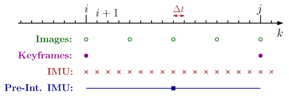
IMU Preintegration

The state of the system at time $k$ is represented by the IMU's orientation, position, velocity, and sensor biases

$$\begin{array}{}\text{(22)}& {\mathrm{x}}_k=[{\mathrm{R}}_{w{b}_k}({\mathbf{q}}_{w{b}_k}),{\mathbf{p}}_{w{b}_k},{\mathbf{v}}_k^w,{\mathbf{b}}_g^{b_k},{\mathbf{b}}_a^{b_k}]\end{array}$$

Let ${\hat{\mathbf{a}}}^b(t)$ and ${\hat{\mathit{\omega }}}^b(t)$ denote the measurements from the three-axis accelerometer and gyroscope, respectively. These are corrupted by noise and time-varying biases:

$$\begin{array}{}\text{(27, 28)}& \begin{array}{rl}{\hat{\mathit{\omega }}}^b(t)& ={\mathit{\omega }}^b(t)+{\mathbf{b}}_g^b(t)+{\mathbf{n}}_g^b(t)\\ {\hat{\mathbf{a}}}^b(t)& ={\mathrm{R}}_{bw}(t)[{\mathbf{a}}^w(t)+{\mathbf{g}}^w]+{\mathbf{b}}_a^b(t)+{\mathbf{n}}_a^b(t)\end{array}\end{array}$$

In this notation, the superscript $w$ refers to the world (inertial) frame, while $b$ denotes the body (sensor) frame. The subscripts $a$ and $g$ refer to the accelerometer and gyroscope, respectively.

The time dirivatives of $\mathrm{R},\mathbf{p},\mathbf{v}$ are given as:

$$\begin{array}{}\text{(29)}& \begin{array}{rl}{\dot{\mathbf{p}}}_{wb}(t)& ={\mathbf{v}}^w(t)\\ {\dot{\mathbf{v}}}^w(t)& ={\mathbf{a}}^w(t)\\ {\dot{\mathrm{R}}}_{wb}(t)& ={\mathrm{R}}_{wb}(t)\cdot \text{Exp}[{\mathit{\omega }}^b(t)]\\ {\dot{\mathbf{q}}}_{wb}(t)& ={\mathbf{q}}_{wb}(t)\otimes \left[\begin{array}{c}0\\ \frac{1}{2}{\mathit{\omega }}^b(t)\end{array}\right]\end{array}\end{array}$$

Using these dynamics, we can express the system state at time $t+\mathrm{\Delta }t$ as follows:

$$\begin{array}{rl}{\mathbf{p}}_{wb}(t+\mathrm{\Delta }t)& ={\mathbf{p}}_{wb}(t)+{\mathbf{v}}^w(t)\cdot \mathrm{\Delta }t+{\iint }_t^{t+\mathrm{\Delta }t}{\mathbf{a}}^w(\tau )\mathrm{d}{\tau }^2\\ & ={\mathbf{p}}_{wb}(t)+{\mathbf{v}}^w(t)\cdot \mathrm{\Delta }t+{\iint }_t^{t+\mathrm{\Delta }t}[{\mathrm{R}}_{wb}(\tau )({\hat{\mathbf{a}}}^b(\tau )-{\mathbf{b}}_a^b(\tau )-{\mathbf{n}}_a^b(\tau ))-{\mathbf{g}}^w]\mathrm{d}{\tau }^2\\ & ={\mathbf{p}}_{wb}(t)+{\mathbf{v}}^w(t)\cdot \mathrm{\Delta }t-\frac{1}{2}{\mathbf{g}}^w\cdot (\mathrm{\Delta }t{)}^2+{\iint }_t^{t+\mathrm{\Delta }t}{\mathrm{R}}_{wb}(\tau )[{\hat{\mathbf{a}}}^b(\tau )-{\mathbf{b}}_a^b(\tau )-{\mathbf{n}}_a^b(\tau )]\mathrm{d}{\tau }^2\\ {\mathbf{v}}^w(t+\mathrm{\Delta }t)& ={\mathbf{v}}^w(t)+{\int }_t^{t+\mathrm{\Delta }t}{\mathbf{a}}^w(\tau )\mathrm{d}\tau \\ & ={\mathbf{v}}^w(t)+{\int }_t^{t+\mathrm{\Delta }t}[{\mathrm{R}}_{wb}(\tau )({\hat{\mathbf{a}}}^b(\tau )-{\mathbf{b}}_a^b(\tau )-{\mathbf{n}}_a^b(\tau ))-{\mathbf{g}}^w]\mathrm{d}{\tau }^2\\ & ={\mathbf{v}}^w(t)-{\mathbf{g}}^w\cdot \mathrm{\Delta }t+{\int }_t^{t+\mathrm{\Delta }t}{\mathrm{R}}_{wb}(\tau )[{\hat{\mathbf{a}}}^b(\tau )-{\mathbf{b}}_a^b(\tau )-{\mathbf{n}}_a^b(\tau )]\mathrm{d}{\tau }^2\\ {\mathrm{R}}_{wb}(t+\mathrm{\Delta }t)& ={\int }_t^{t+\mathrm{\Delta }t}{\mathrm{R}}_{wb}(\tau )\cdot \text{Exp}({\mathit{\omega }}^b(\tau ))\mathrm{d}\tau \\ & ={\int }_t^{t+\mathrm{\Delta }t}{\mathrm{R}}_{wb}(\tau )\cdot \text{Exp}({\hat{\mathit{\omega }}}^b(\tau )-{\mathbf{b}}_g^b(\tau )-{\mathbf{n}}_g^b(\tau ))\mathrm{d}\tau \\ {\mathbf{q}}_{wb}(t+\mathrm{\Delta }t)& ={\int }_t^{t+\mathrm{\Delta }t}{\mathbf{q}}_{wb}(\tau )\otimes \left[\begin{array}{c}0\\ \frac{1}{2}{\mathit{\omega }}^b(t)\end{array}\right]\mathrm{d}\tau \\ & ={\int }_t^{t+\mathrm{\Delta }t}{\mathbf{q}}_{wb}(\tau )\otimes \left[\begin{array}{c}0\\ \frac{1}{2}({\hat{\mathit{\omega }}}^b(\tau )-{\mathbf{b}}_g^b(\tau )-{\mathbf{n}}_g^b(\tau ))\end{array}\right]\mathrm{d}\tau \end{array}$$

However, recomputing ${\mathrm{R}}_{wb}(\tau )$ at each step leads to repeated integration and unnecessary computational cost. To mitigate this, we use the identity:

$${\mathrm{R}}_{wb}(\tau )={\mathrm{R}}_{w{b}_t}\cdot {\mathrm{R}}_{b_{t}b}(\tau )$$

This allows us to factor out ${\mathrm{R}}_{w{b}_i}$ from the integrals over the interval $[t_i,t_j]$, resulting in:

$$\begin{array}{rl}{\mathrm{R}}_{w{b}_j}& ={\mathrm{R}}_{w{b}_i}\cdot {\int }_{t_i}^{t_j}{\mathrm{R}}_{b_{i}b}(\tau )\cdot \text{Exp}({\hat{\mathit{\omega }}}^b(\tau )-{\mathbf{b}}_g^b(\tau )-{\mathbf{n}}_g^b(\tau ))\mathrm{d}\tau \\ {\mathbf{q}}_{w{b}_j}& ={\mathbf{q}}_{w{b}_i}\otimes {\int }_{t_i}^{t_j}{\mathbf{q}}_{b_{i}b}(\tau )\otimes \left[\begin{array}{c}0\\ \frac{1}{2}({\hat{\mathit{\omega }}}^b(\tau )-{\mathbf{b}}_g^b(\tau )-{\mathbf{n}}_g^b(\tau ))\end{array}\right]\mathrm{d}\tau \\ {\mathbf{p}}_{w{b}_j}& ={\mathbf{p}}_{w{b}_i}+{\mathbf{v}}_i^w\cdot \mathrm{\Delta }t-\frac{1}{2}{\mathbf{g}}^w\cdot (\mathrm{\Delta }t{)}^2+{\mathrm{R}}_{w{b}_i}{\iint }_{t_i}^{t_j}{\mathrm{R}}_{b_{i}b}(\tau )[{\hat{\mathbf{a}}}^b(\tau )-{\mathbf{b}}_a^b(\tau )-{\mathbf{n}}_a^b(\tau )]\mathrm{d}{\tau }^2\\ {\mathbf{v}}_j^w& ={\mathbf{v}}_i^w-{\mathbf{g}}^w\cdot \mathrm{\Delta }t+{\mathrm{R}}_{w{b}_i}{\int }_{t_i}^{t_j}{\mathrm{R}}_{b_{i}b}(\tau )[{\hat{\mathbf{a}}}^b(\tau )-{\mathbf{b}}_a^b(\tau )-{\mathbf{n}}_a^b(\tau )]\mathrm{d}\tau \end{array}$$

We define the following preintegrated terms:

$$\begin{array}{rl}{\mathit{\alpha }}_{b_i{b}_j}& ={\iint }_{t_i}^{t_j}{\mathrm{R}}_{b_{i}b}(\tau )[{\hat{\mathbf{a}}}^b(\tau )-{\mathbf{b}}_a^b(\tau )-{\mathbf{n}}_a^b(\tau )]\mathrm{d}{\tau }^2\\ {\mathit{\beta }}_{b_i{b}_j}& ={\int }_{t_i}^{t_j}{\mathrm{R}}_{b_{i}b}(\tau )[{\hat{\mathbf{a}}}^b(\tau )-{\mathbf{b}}_a^b(\tau )-{\mathbf{n}}_a^b(\tau )]\mathrm{d}\tau \\ {\mathit{\gamma }}_{b_i{b}_j}& ={\int }_{t_i}^{t_j}{\mathrm{R}}_{b_{i}b}(\tau )\cdot \text{Exp}({\hat{\mathit{\omega }}}^b(\tau )-{\mathbf{b}}_g^b(\tau )-{\mathbf{n}}_g^b(\tau ))\mathrm{d}\tau \end{array}$$

Thus, the final update equations become:

$$\begin{array}{rl}{\mathbf{p}}_{w{b}_j}& ={\mathbf{p}}_{w{b}_i}+{\mathbf{v}}_i^w\mathrm{\Delta }t-\frac{1}{2}{\mathbf{g}}^w\mathrm{\Delta }{t}^2+{\mathrm{R}}_{w{b}_i}{\mathit{\alpha }}_{b_i{b}_j}\\ {\mathbf{v}}_j^w& ={\mathbf{v}}_i^w-{\mathbf{g}}^w\mathrm{\Delta }t+{\mathrm{R}}_{w{b}_i}{\mathit{\beta }}_{b_i{b}_j}\\ {\mathrm{R}}_{w{b}_j}& ={\mathrm{R}}_{w{b}_i}\cdot {\mathit{\gamma }}_{b_i{b}_j}\end{array}$$

Finally, since the gyroscope and accelerometer biases are modeled as Gaussian white noise processes with zero mean:

$$\dot{\mathbf{b}}\sim \mathcal{N}(0,\mathrm{\Sigma })$$

we assume that the bias remains approximately constant between two consecutive time steps:

$${\mathbf{b}}_g^{b_i}={\mathbf{b}}_g^{b_j},{\mathbf{b}}_a^{b_i}={\mathbf{b}}_a^{b_j},\mathrm{\forall }i,j$$