Factor Graph for Pose Estimation

Slide: Overview of factor graphs in pose estimation, emphasizing their benefits over Kalman Filters for handling complex dependencies. Covers dynamic Bayesian networks, information forms, and smoothing for efficient state estimation.

Kalman Filter

Markov Chain

The classic Kalman Filter corresponds to a simple Markov Chain:

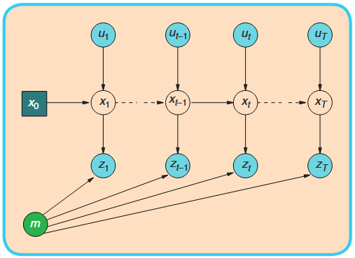
Core Assumptions:

• Markov Property: The current state $x_k$ depends only on the immediate previous state $x_{k-1}$ and input $u_k$
• Conditional Independence: Given the current state $x_k$, the observation $y_k$​ is independent of all other states and observations.

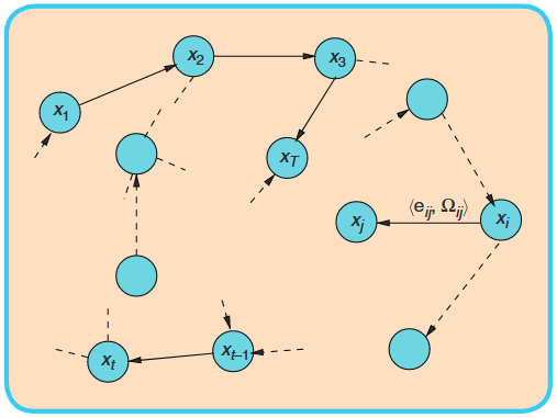
Scenario 1: Spatio-Temporal Constraints

A robot revisits a location, observing the same landmark $l$ at two different times, $k_1$​ and $k_2$:

$$\underset{\text{obs. }l}{x_{k_1}}\to x_{k_1+1}\to \cdots x_{k_2-1}\to \underset{\text{obs. }l}{x_{k_2}}$$

These two observations create a direct constraint between pose $x_{k_1}$​​ and pose $x_{k_2}$​​. In the Kalman Filter, this connection is not direct. We need a way to directly link $x_{k_1}$ and $x_{k_2}$.

Scenario 2: Physical Constraints

When tracking multiple objects, they may be subject to physical interaction constraints

$$\begin{array}{r}\text{Object A: }{x}_0^A\to \underset{\text{interact with B}}{\underbrace{x_1^A\to x_2^A}}\to \cdots \\ \text{Object B: }{x}_0^B\to \underset{\text{interact with A}}{\underbrace{x_1^B\to x_2^B}}\to \cdots \end{array}$$

The Kalman Filter, designed for a single Markov chain, cannot natively represent this cross-object dependency.

Factor Graph

Dynamic Bayesian Networks

Dynamic Bayesian Networks (DBNs) provide a more flexible framework than a simple Markov chain for representing probabilistic dependencies across time.

Extensions:

1. Arbitrary Time-Span Dependencies: States can depend on states several steps back.
2. Complex Inter-Variable Constraints: Multiple variables within a time slice can be interconnected.
3. Hierarchical State Representations: States can be decomposed into sub-states with their own dependencies.

Dynamic Bayesian Networks (cont.)

It is a bipartite graph consisting of two types of nodes:

1. Variable Nodes: Represent the unknown quantities we wish to estimate.
2. Factor Nodes: Represent a constraint or a measurement on the set of variables they are connected to.

Goal: Find the most probable assignment of the variables that maximizes the product of all factors.

$${\mathbf{X}}^{\ast }=\arg \underset{\mathbf{X}}{max}\prod _i{f}_i({\mathcal{X}}_i)$$

Under Gaussian assumptions, this becomes a nonlinear least-squares problem:

$${\mathbf{X}}^{\ast }=\arg \underset{\mathbf{X}}{min}\sum _i||h_i({\mathcal{X}}_i)-z_i|{|}_{{\mathbf{S}}_i}^2$$

Unified View

The Dual Information Form

$$p(\mathit{\alpha },\mathit{\beta })=\mathcal{N}(\left[\begin{array}{c}{\mathit{\mu }}_{\mathit{\alpha }}\\ {\mathit{\mu }}_{\mathit{\beta }}\end{array}\right],\left[\begin{array}{cc}{\mathbf{\Sigma }}_{\mathit{\alpha }\mathit{\alpha }}& {\mathbf{\Sigma }}_{\mathit{\alpha }\mathit{\beta }}\\ {\mathbf{\Sigma }}_{\mathit{\beta }\mathit{\alpha }}& {\mathbf{\Sigma }}_{\mathit{\beta }\mathit{\beta }}\end{array}\right])={\mathcal{N}}^{-1}(\left[\begin{array}{c}{\mathit{\eta }}_{\mathit{\alpha }}\\ {\mathit{\eta }}_{\mathit{\beta }}\end{array}\right],\left[\begin{array}{cc}{\mathbf{\Lambda }}_{\mathit{\alpha }\mathit{\alpha }}& {\mathbf{\Lambda }}_{\mathit{\alpha }\mathit{\beta }}\\ {\mathbf{\Lambda }}_{\mathit{\beta }\mathit{\alpha }}& {\mathbf{\Lambda }}_{\mathit{\beta }\mathit{\beta }}\end{array}\right])$$

Operation	Covariance Form	Information Form
Marginalization $p(\mathit{\alpha })=\int p(\mathit{\alpha },\mathit{\beta })\mathrm{d}\mathit{\beta }$	$\begin{array}{rl}\mathit{\mu }& ={\mathit{\mu }}_{\mathit{\alpha }}\\ \mathbf{\Sigma }& ={\mathbf{\Sigma }}_{\mathit{\alpha }\mathit{\alpha }}\end{array}$	$\begin{array}{rl}\mathit{\eta }& ={\mathit{\eta }}_{\mathit{\alpha }}-{\mathbf{\Lambda }}_{\mathit{\alpha }\mathit{\beta }}{\mathbf{\Lambda }}_{\mathit{\beta }\mathit{\beta }}^{-1}{\mathit{\eta }}_{\mathit{\beta }}\\ \mathbf{\Lambda }& ={\mathbf{\Lambda }}_{\mathit{\alpha }\mathit{\alpha }}-{\mathbf{\Lambda }}_{\mathit{\alpha }\mathit{\beta }}{\mathbf{\Lambda }}_{\mathit{\beta }\mathit{\beta }}^{-1}{\mathbf{\Lambda }}_{\mathit{\beta }\mathit{\alpha }}\end{array}$
Conditioning $p(\mathit{\alpha }\mid \mathit{\beta })=p(\mathit{\alpha },\mathit{\beta })/p(\mathit{\beta })$	$\begin{array}{rl}{\mathit{\mu }}^{\prime }& ={\mathit{\mu }}_{\mathit{\alpha }}+{\mathbf{\Sigma }}_{\mathit{\alpha }\mathit{\beta }}{\mathbf{\Sigma }}_{\mathit{\beta }\mathit{\beta }}^{-1}(\mathit{\beta }-{\mathit{\mu }}_{\mathit{\beta }})\\ {\mathbf{\Sigma }}^{\prime }& ={\mathbf{\Sigma }}_{\mathit{\alpha }\mathit{\alpha }}-{\mathbf{\Sigma }}_{\mathit{\alpha }\mathit{\beta }}{\mathbf{\Sigma }}_{\mathit{\beta }\mathit{\beta }}^{-1}{\mathbf{\Sigma }}_{\mathit{\beta }\mathit{\alpha }}\end{array}$	$\begin{array}{rl}{\mathit{\eta }}^{\prime }& ={\mathit{\eta }}_{\mathit{\alpha }}-{\mathbf{\Lambda }}_{\mathit{\alpha }\mathit{\beta }}\mathit{\beta }\\ {\mathbf{\Lambda }}^{\prime }& ={\mathbf{\Lambda }}_{\mathit{\alpha }\mathit{\alpha }}\end{array}$

The Dual Information Filter

	Kalman Filter	Information Filter
Prediction Step	$\begin{array}{rl}{\mathit{\mu }}_{t|t-1}& ={\mathbf{A}}_t{\mathit{\mu }}_{t-1}\\ {\mathbf{\Sigma }}_{t|t-1}& ={\mathbf{A}}_t{\mathbf{\Sigma }}_{t-1}{\mathbf{A}}_t^{\mathrm{\top }}+{\mathbf{Q}}_t\end{array}$	$\begin{array}{rl}{\mathbf{\Lambda }}_{t|t-1}& =({\mathbf{A}}_t{\mathbf{\Lambda }}_{t-1}^{-1}{\mathbf{A}}_t^{\mathrm{\top }}+{\mathbf{Q}}_t{)}^{-1}\\ {\mathit{\eta }}_{t|t-1}& ={\mathbf{\Lambda }}_{t|t-1}{\mathbf{A}}_t{\mathbf{\Lambda }}_{t-1}^{-1}{\mathit{\eta }}_{t-1}\end{array}$
Update Step	$\begin{array}{rl}{\mathbf{K}}_t& ={\mathbf{\Sigma }}_{t|t-1}{\mathbf{H}}_t^{\mathrm{\top }}({\mathbf{H}}_t{\mathbf{\Sigma }}_{t|t-1}{\mathbf{H}}_t^{\mathrm{\top }}+{\mathbf{R}}_t{)}^{-1}\\ {\mathit{\mu }}_t& ={\mathit{\mu }}_{t|t-1}+{\mathbf{K}}_t({\mathbf{z}}_t-{\mathbf{H}}_t{\mathit{\mu }}_{t|t-1})\\ {\mathbf{\Sigma }}_t& =(\mathbf{I}-{\mathbf{K}}_t{\mathbf{H}}_t){\mathbf{\Sigma }}_{t|t-1}\end{array}$	$\begin{array}{rl}{\mathbf{\Lambda }}_t& ={\mathbf{\Lambda }}_{t|t-1}+{\mathbf{H}}_t^{\mathrm{\top }}{\mathbf{R}}_t^{-1}{\mathbf{H}}_t\\ {\mathit{\eta }}_t& ={\mathit{\eta }}_{t|t-1}+{\mathbf{H}}_t^{\mathrm{\top }}{\mathbf{R}}_t^{-1}{\mathbf{z}}_t\end{array}$

Factor Graph with Information Form

The global nonlinear optimization problem

$${\mathbf{X}}^{\ast }=\arg \underset{\mathbf{X}}{min}\sum _i||h_i({\mathcal{X}}_i)-z_i|{|}_{{\mathbf{S}}_i}^2$$

can be linearized at current estimation ${\mathbf{X}}_0$:

$$h_i({\mathcal{X}}_i)\approx h_i({\mathcal{X}}_{i,0})+{\mathbf{J}}_i\cdot \delta {\mathcal{X}}_i$$

where:

• ${\mathbf{J}}_i=\frac{\partial h_i}{\partial {\mathcal{X}}_i}{|}_{{\mathcal{X}}_{i,0}}$ is the Jacobian matrix of measurement function $h_i$
• ${\mathbf{r}}_i=z_i-h_i({\mathcal{X}}_{i,0})$ is the residual vector

Factor Graph with Information Form (cont.)

Local Information Form	Global Information Form
$\begin{array}{rl}{\mathbf{\Lambda }}_i& ={\mathbf{J}}_i^{\mathrm{\top }}{\mathbf{S}}_i^{-1}{\mathbf{J}}_i\\ {\mathit{\eta }}_i& ={\mathbf{J}}_i^{\mathrm{\top }}{\mathbf{S}}_i^{-1}{\mathbf{r}}_i\end{array}$	$\begin{array}{rl}\mathbf{\Lambda }& =\sum _i{\mathbf{A}}_i^{\mathrm{\top }}{\mathbf{\Lambda }}_i{\mathbf{A}}_i\\ \mathit{\eta }& =\sum _i{\mathbf{A}}_i^{\mathrm{\top }}{\mathit{\eta }}_i\end{array}$

where ${\mathbf{A}}_i$ is the selection matrix that maps local variables ${\mathcal{X}}_i$ to the global state vector $\mathbf{X}$.

The optimal update is then:

$${\mathbf{X}}^{\ast }={\mathbf{X}}_0+(\mathbf{\Lambda }{)}^{-1}\mathit{\eta }$$

From Filtering to Smoothing

Kalman Filter, Information Filter, and Factor Graph are fundamentally solving the same problem: state estimation under Gaussian assumptions. They are probabilistically equivalent.

Despite mathematical equivalence, FG-based smoothing dominates modern applications because:

1. It naturally encodes arbitrary constraints;
2. It exploits sparse structure for efficient solving;
3. It's batch-based update enabling non-linear optimization;
4. It corrects past states by future evidence.