The Duality and the Failure of LQG Control

Slide: Explore the duality between state observers and feedback controllers, focusing on KF and LQR. Understand why combining the "optimal observer" with the "optimal controller" might fail. Inspired by Dominikus Noll's page "A generalization of the Linear Quadratic Gaussian Loop Transfer Recovery procedure (LQG/LTR)".

Introduction

System Model

Consider a $n$-th order linear time-invariant (LTI) discrete-time dynamic system with $m$-dimensional input and $p$-dimensional output:

$$\begin{array}{rlr}{x}_{k+1}& =A{x}_k+B{u}_k+{\omega }_k,& {\omega }_k\sim \mathcal{N}(0,W_k)\\ y_k& =C{x}_k+{\nu }_k,& {\nu }_k\sim \mathcal{N}(0,V_k)\end{array}$$

• $x_k\in {\mathbb{R}}^n$: state vector at time step $k$
• $u_k\in {\mathbb{R}}^m$: control input vector at time step $k$
• $y_k\in {\mathbb{R}}^p$: measurement vector at time step $k$
• $A\in {\mathbb{R}}^{n\times n}$: state transition matrix
• $B\in {\mathbb{R}}^{n\times m}$: control input matrix
• $C\in {\mathbb{R}}^{p\times n}$: observation matrix

Controllability

A LTI system is said to be controllable if,

$$\mathrm{\forall }{x}_0,x^{\ast },\mathrm{\exists }k>0,{\mathbf{u}}_k=[u_{k-1},\cdots ,u_1,u_0],\text{such that}{x}_k=x^{\ast }.$$

This is equivalent to $\text{rank}(M_c)=n$, where $M_c=[B,AB,A^{2}B,\dots ,A^{n-1}B]\in {\mathbb{R}}^{n\times nm}$ is the controllability matrix.

$$\begin{array}{rl}{x}_n& =A{x}_{n-1}+B{u}_{n-1}\\ & =A(A{x}_{n-2}+B{u}_{n-2})+B{u}_{n-1}\\ & =A^2{x}_{n-2}+AB{u}_{n-2}+B{u}_{n-1}\\ & =A^n{x}_0+A^{n-1}B{u}_0+\cdots +AB{u}_{n-2}+B{u}_{n-1}\\ & =A^n{x}_0+M_c{\mathbf{u}}_n\end{array}$$$${\mathbf{u}}_n=M_c^{\mathrm{\top }}(M_c{M}_c^{\mathrm{\top }}{)}^{-1}(x^{\ast }-A^n{x}_0)$$

Observability

A LTI system is said to be observable if,

$$\mathrm{\forall }{x}_0\in {\mathbb{R}}^n\mathrm{\exists }k>0,{\mathbf{y}}_{\mathbf{k}}=[y_0,y_1,\dots ,y_{k-1}{]}^{\mathrm{\top }}\Rightarrow x_0.$$

This is equivalent to $\text{rank}(M_o)=n$, where $M_o=[C^{\mathrm{\top }},(CA{)}^{\mathrm{\top }},(C{A}^2{)}^{\mathrm{\top }},\dots ,(C{A}^{n-1}{)}^{\mathrm{\top }}{]}^{\mathrm{\top }}\in {\mathbb{R}}^{np\times n}$ is the observability matrix.

$$\begin{array}{rl}{y}_0& =C{x}_0\\ y_1& =C{x}_1=CA{x}_0\\ & ⋮\\ y_{n-1}& =C{A}^{n-1}{x}_0\end{array}\Rightarrow {\mathbf{y}}_n=\left[\begin{array}{c}{y}_0\\ y_1\\ ⋮\\ y_{n-1}\end{array}\right]=\left[\begin{array}{c}C\\ CA\\ ⋮\\ C{A}^{n-1}\end{array}\right]x_0=M_o{x}_0$$$$x_0=(M_o^{\mathrm{\top }}{M}_o{)}^{-1}{M}_o^{\mathrm{\top }}{\mathbf{y}}_n$$

The Optimality

Optimal Estimator: Kalman Filter

Goal:

$$\underset{{\hat{x}}_{k|k}}{min}\mathbb{E}[(x_k-{\hat{x}}_{k|k})(x_k-{\hat{x}}_{k|k}{)}^{\mathrm{\top }}\mid y_1,\dots ,y_k]$$

Solution:

$$\begin{array}{rl}{\hat{x}}_{k|k-1}& =A{\hat{x}}_{k-1|k-1}+B{u}_{k-1}\\ {\hat{P}}_{k|k-1}& =A{\hat{P}}_{k-1|k-1}{A}^{\mathrm{\top }}+W_{k-1}\\ K_k& ={\hat{P}}_{k|k-1}{C}^{\mathrm{\top }}(C{\hat{P}}_{k|k-1}{C}^{\mathrm{\top }}+V_k{)}^{-1}\\ {\hat{x}}_{k|k}& ={\hat{x}}_{k|k-1}+K_k(y_k-C{\hat{x}}_{k|k-1})\\ {\hat{P}}_{k|k}& ={\hat{P}}_{k|k-1}-K_{k}C{\hat{P}}_{k|k-1}=({\hat{P}}_{k|k-1}^{-1}+C^{\mathrm{\top }}{V}_k^{-1}C{)}^{-1}\end{array}$$

Optimal Regulator: LQR

Goal:

$$\underset{\{u_k\}}{min}\mathbb{E}[x_N^{\mathrm{\top }}{Q}_N{x}_N+\sum _{k=0}^{N-1}(x_k^{\mathrm{\top }}{Q}_k{x}_k+u_k^{\mathrm{\top }}{R}_k{u}_k)]$$

Solution:

$$\begin{array}{rl}{S}_N& =Q_N\\ L_k& =(R_k+B_k^{\mathrm{\top }}{S}_{k+1}{B}_k{)}^{-1}{B}_k^{\mathrm{\top }}{S}_{k+1}{A}_k\\ S_k& =Q_k+A_k^{\mathrm{\top }}{S}_{k+1}(A_k-B_k{L}_k)\\ u_k& =-L_k{x}_k\end{array}$$

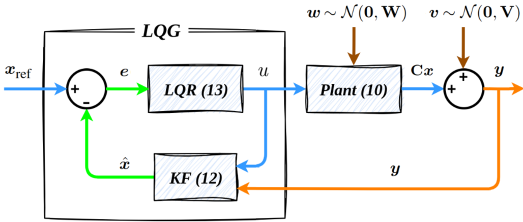
Linear Quadratic Gaussian (LQG)

The separation principle states that the design of the optimal controller and the optimal observer can be separated. The optimal control law is given by:

$$u_k=-L_k{\hat{x}}_{k|k}$$

where ${\hat{x}}_{k|k}$ is the state estimate provided by the Kalman filter.

'Inertial-Based LQG Control' by Daniel Engelsman

The Duality

The Duality in Control Theory

Controllability vs Observability For the original system $\mathrm{\Sigma }=(A,B,C)$, the dual system is defined as ${\mathrm{\Sigma }}^{\ast }=(A^{\mathrm{\top }},C^{\mathrm{\top }},B^{\mathrm{\top }})$.

• $\mathrm{\Sigma }$ is controllable $\iff$ ${\mathrm{\Sigma }}^{\ast }$ is observable
• $\mathrm{\Sigma }$ is observable $\iff$ ${\mathrm{\Sigma }}^{\ast }$ is controllable

Controller vs Observer

• Feedback controller $u_k=-L_k{x}_k$ "suppresses" the state deviation $x_k$ through inputs
• State observer ${\hat{x}}_{k|k}={\hat{x}}_{k|k-1}+K_k(y_k-C{\hat{x}}_{k|k-1})$ "corrects" the state estimate ${\hat{x}}_{k|k}$ through measurements
• The design of $L_k$ and $K_k$ are dual problems

The Duality in LQR and Kalman Filter (Optimization)

Optimization formulation of LQR:

$$\underset{x_{1:N},u_{1:N-1}}{min}{x}_N^{\mathrm{\top }}{Q}_N{x}_N+\sum _{k=0}^{N-1}[x_k^{\mathrm{\top }}{Q}_k{x}_k+u_k^{\mathrm{\top }}{R}_k{u}_k]$$

Optimization formulation of Kalman Filter:

$$\underset{x_{1:N},{\omega }_{1:N-1}}{min}(x_0-{\hat{x}}_{0|0}{)}^{\mathrm{\top }}{P}_0^{-1}(x_0-{\hat{x}}_{0|0})+\sum _{k=0}^{N-1}[(y_k-C{x}_k{)}^{\mathrm{\top }}{V}_k^{-1}(y_k-C{x}_k)+{\omega }_k^{\mathrm{\top }}{W}_k^{-1}{\omega }_k]$$

subject to $x_{k+1}=A{x}_k+B{u}_k+{\omega }_k$.

Duality:

$$A\leftrightarrow A^{\mathrm{\top }},B\leftrightarrow C^{\mathrm{\top }},Q\leftrightarrow W,R\leftrightarrow V$$

The Duality in LQR and Kalman Filter (Riccati)

Riccati Equation in LQR:

$$\{\begin{array}{l}{L}_k=(R_k+B_k^{\mathrm{\top }}{S}_{k+1}{B}_k{)}^{-1}{B}_k^{\mathrm{\top }}{S}_{k+1}{A}_k\\ S_k=Q_k+A_k^{\mathrm{\top }}{S}_{k+1}(A_k-B_k{L}_k)\end{array}$$$$S=A^{\mathrm{\top }}SA+Q-A^{\mathrm{\top }}SB(B^{\mathrm{\top }}SB+R{)}^{-1}{B}^{\mathrm{\top }}SA$$

Riccati Equation in Kalman Filter:

$$\{\begin{array}{l}{\hat{P}}_{k|k-1}=A{\hat{P}}_{k-1|k-1}{A}^{\mathrm{\top }}+W_{k-1}\\ K_k={\hat{P}}_{k|k-1}{C}^{\mathrm{\top }}(C{\hat{P}}_{k|k-1}{C}^{\mathrm{\top }}+V_k{)}^{-1}\\ {\hat{P}}_{k|k}={\hat{P}}_{k|k-1}-K_{k}C{\hat{P}}_{k|k-1}=({\hat{P}}_{k|k-1}^{-1}+C^{\mathrm{\top }}{V}_k^{-1}C{)}^{-1}\end{array}$$$$P=AP{A}^{\mathrm{\top }}+W-AP{C}^{\mathrm{\top }}(CP{C}^{\mathrm{\top }}+V{)}^{-1}CP{A}^{\mathrm{\top }}$$

Duality:

$$A\leftrightarrow A^{\mathrm{\top }},B\leftrightarrow C^{\mathrm{\top }},Q\leftrightarrow W,R\leftrightarrow V,S\leftrightarrow P$$

The Failure

The Paradox of Optimality

LQR Robustness (SISO systems):

• $\ge 60\mathrm{deg}$ Phase Margin
• $\ge 6\text{ dB}$ Gain Margin
• Infinite gain reduction margin

Kalman Filter Robustness:

• Dual robustness properties at sensor output
• Excellent margins against sensor errors

The Fundamental Trade-Off

LQR's Need for High-Gain Feedback:

• Large Q & Small R
• Excellent stability margins

KF's Need for High-Gain Feedback:

• Large W & Small V
• Prompt response to new measurements

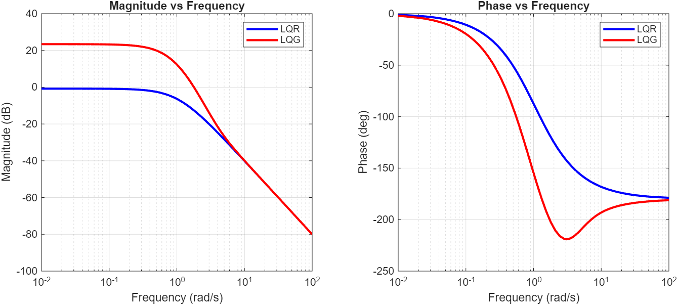
Optimizing for individual robustness leads to a fragile combined LQG system.

The Destructive Feedback Loop:

1. High-gain L reacts aggressively to state deviations
2. High-gain K amplifies sensor noise
3. This creates a positive feedback loop
4. Resulting in potential instability of the system

No stability guarantee for imperfect models, leading to the development of $H_{\mathrm{\infty }}$ Control