CoTiMo Planner Code Report

Collision-Free Smooth Path Generation

Cubic Spline

For a group of certain points $(x_{0,1},x_{0,2},\cdots ,x_{0,m}),(x_{1,1},x_{1,2},\cdots ,x_{1,m}),(x_{2,1},x_{2,2},\cdots ,x_{2,m}),\cdots ,(x_{n,1},x_{n,2},\cdots ,x_{n,m})$, we want to find a smooth enough curve that passes all these points to achieve the interpolation goal. To do so, we can use piecewise cubic functions to fitting the points.

Let's talk about a specific dimention $k$ first. To simplify the denotation, we let $x_i=x_{i,k}$. For a set of $n+1$ points $(x_{0,k},x_{1,k},x_{2,k},\cdots ,x_{n,k})$ and for the $i$-th piece of the spline, we can represent it by

$$q_i(s)=a_i{s}^3+b_i{s}^2+c_{i}s+d_i,s\in [0,1],i=0,1,\cdots ,n-1$$

To ensure the smooth of the curve, we write down the constraints,

$$\{\begin{array}{l}{q}_{i-1}(1)=q_i(0)=x_i\\ q_{i-1}^{\prime }(1)=q_i^{\prime }(0)\\ q_{i-1}^{″}(1)=q_i^{″}(0)\end{array}$$

Apply $a_i,b_i,c_i,d_i$ to the constraints, we get

$$\{\begin{array}{l}{a}_{i-1}+b_{i-1}+c_{i-1}+d_{i-1}=d_i\\ 3a_{i-1}+2b_{i-1}+c_{i-1}=c_i\\ 6a_{i-1}+2b_{i-1}=2b_i\end{array}$$

So we can get the following expressions

$$\{\begin{array}{l}{a}_i=x_{i+2}-2x_{i+1}+x_i\\ b_i=-x_{i+2}+2x_{i+1,k}-x_i\\ c_i=x_{i+1}-x_i\\ d_i=x_i\end{array},i=1,2,\cdots ,n-1$$

In open loop case, assume stationary boundary $q_0^{\prime }(0)=0,q_{n-1}^{\prime }(1)=0$, which is $c_0=0,3a_{n-1}+2b_{n-1}+c_{n-1}=0$.

You can also regard $x_{n+2}$ as $x_{n+1}$, so that $x_{n+2}-2x_{n+1}+x_n=-x_{n+1}+x_n$

Convert the expressions to vector form, we have

$$\left[\begin{array}{c}{a}_0\\ a_1\\ a_2\\ a_3\\ ⋮\\ a_{n-2}\\ a_{n-1}\end{array}\right]=\left[\begin{array}{cccccccc}2& -3& 1& 0& \cdots & 0& 0& 0\\ 0& 1& -2& 1& \cdots & 0& 0& 0\\ 0& 0& 1& -2& \cdots & 0& 0& 0\\ 0& 0& 0& 1& \cdots & 0& 0& 0\\ ⋮& ⋮& ⋮& ⋮& \ddots & ⋮& ⋮& ⋮\\ 0& 0& 0& 0& \cdots & 1& -2& 1\\ 0& 0& 0& 0& \cdots & 0& 1& -1\end{array}\right]\left[\begin{array}{c}{x}_0\\ x_1\\ x_2\\ x_3\\ ⋮\\ x_{n-2}\\ x_{n-1}\\ x_n\end{array}\right]$$$$\left[\begin{array}{c}{b}_0\\ b_1\\ b_2\\ b_3\\ ⋮\\ b_{n-2}\\ b_{n-1}\end{array}\right]=\left[\begin{array}{cccccccc}-3& 4& -1& 0& \cdots & 0& 0& 0\\ 0& -1& 2& -1& \cdots & 0& 0& 0\\ 0& 0& -1& 2& \cdots & 0& 0& 0\\ 0& 0& 0& -1& \cdots & 0& 0& 0\\ ⋮& ⋮& ⋮& ⋮& \ddots & ⋮& ⋮& ⋮\\ 0& 0& 0& 0& \cdots & -1& 2& -1\\ 0& 0& 0& 0& \cdots & 0& -1& 1\end{array}\right]\left[\begin{array}{c}{x}_0\\ x_1\\ x_2\\ x_3\\ ⋮\\ x_{n-2}\\ x_{n-1}\\ x_n\end{array}\right]$$$$\left[\begin{array}{c}{c}_0\\ c_1\\ c_2\\ c_3\\ ⋮\\ c_{n-2}\\ c_{n-1}\end{array}\right]=\left[\begin{array}{cccccccc}0& 0& 0& 0& \cdots & 0& 0& 0\\ 0& -1& 1& 0& \cdots & 0& 0& 0\\ 0& 0& -1& 1& \cdots & 0& 0& 0\\ 0& 0& 0& -1& \cdots & 0& 0& 0\\ ⋮& ⋮& ⋮& ⋮& \ddots & ⋮& ⋮& ⋮\\ 0& 0& 0& 0& \cdots & -1& 1& 0\\ 0& 0& 0& 0& \cdots & 0& -1& 1\end{array}\right]\left[\begin{array}{c}{x}_0\\ x_1\\ x_2\\ x_3\\ ⋮\\ x_{n-2}\\ x_{n-1}\\ x_n\end{array}\right]$$$$\left[\begin{array}{c}{d}_0\\ d_1\\ d_2\\ d_3\\ ⋮\\ d_{n-2}\\ d_{n-1}\end{array}\right]=\left[\begin{array}{cccccccc}1& 0& 0& 0& \cdots & 0& 0& 0\\ 0& 1& 0& 0& \cdots & 0& 0& 0\\ 0& 0& 1& 0& \cdots & 0& 0& 0\\ 0& 0& 0& 1& \cdots & 0& 0& 0\\ ⋮& ⋮& ⋮& ⋮& \ddots & ⋮& ⋮& ⋮\\ 0& 0& 0& 0& \cdots & 1& 0& 0\\ 0& 0& 0& 0& \cdots & 0& 1& 0\end{array}\right]\left[\begin{array}{c}{x}_0\\ x_1\\ x_2\\ x_3\\ ⋮\\ x_{n-2}\\ x_{n-1}\\ x_n\end{array}\right]$$

For every dimension in $x$, we would obtain four vector $a,b,c,d$

Minimize Stretch Energy

Then, we can define energy function by acceleration

$$Energy(x_0,x_1,\cdots ,x_n)=\sum _{i=1}^{n-1}{\int }_0^1||q_i^{″}(s)|{|}_1\mathrm{d}s$$

But in practice, I use the following formula

$$Energy(x_0,x_1,\cdots ,x_n)=\sum _{i=1}^{n-1}||x_{i-1}-2x_i+x_{i+1}|{|}^2$$

Collision Free

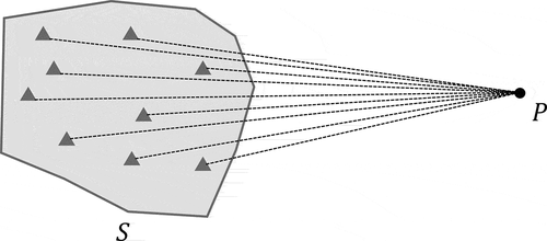
We want to avoid our robot get crashed into the obstacle. So that we also need to define a potential function.

First, we need to calculate the distance between the robot and the obstacle. Which is find a point $o$ in obstacle ($Ao\le b$), to minimize the distance from robot $x$ to point $o$

$$\begin{array}{rl}min& ||o-x|{|}^2\\ \text{s.t.}& Ao\le b\end{array}$$$$\begin{array}{rl}min& o^{T}o-2x^{T}o+x^{T}x\\ \text{s.t.}& Ao\le \text{b}\end{array}$$

By SOCP, we can obtain the distance vector

$$d(x)={\left[\begin{array}{c}d(x,o_1),d(x,o_2),\cdots ,d(x,o_m)\end{array}\right]}^T$$

And the potential function would be defined as below

$$Potential(x_0,x_1,\cdots ,x_n)=\sum _{i=0}^n\exp (||d(x_i)|{|}_{\mathrm{\infty }})$$

Loss Function

$$Loss(x_0,x_1,\cdots ,x_n)=\eta \cdot Energy(x_0,x_1,\cdots ,x_n)+(1-\eta )\cdot Potential(x_0,x_1,\cdots ,x_n)$$

Finally, we convert the problem to an optimization problem, we can use Line Search, Quasi Newton, LBFGS, or Newton-CG to solve it.

$$\underset{x_0,x_1,\cdots ,x_n}{min}Loss(x_0,x_1,\cdots ,x_n)$$

In practice, I add some trick to make the optimizer more stable. Additional to five different $\eta$, I introduce sigmoid function in update step.

$$\sigma (x)=\frac{1}{1+e^{-x}}=\frac{e^x}{1+e^x}=1-\sigma (-x)$$$$x^{k+1}=x^k-{\eta }_k[2\cdot \sigma (\mathrm{\nabla }Loss(x))-1]$$

Time Optimal Path Parameterization

Continuous Case

After optimizing the control points $x_0,x_1,\cdots ,x_n$, we get a spline $q$ uniquely determined by arc-length $s$.

Then the optimal time $T$ is integrated by

$$T={\int }_0^{T}1\mathrm{d}t={\int }_0^L\frac{1}{\frac{\mathrm{d}s}{\mathrm{d}t}}\mathrm{d}s$$

Additional to $q(s)$, $\frac{\mathrm{d}q}{\mathrm{d}s}$ and $\frac{{\mathrm{d}}^{2}q}{\mathrm{d}{s}^2}$ are also known. Because the cubic spline is second order differentiable.

We also have velocity constraint,

$$-v_{max}\le v\le v_{max}$$

acceleration constraint,

$$-a_{max}\le a\le a_{max}$$

and always move forward constraint

$$\frac{\mathrm{d}s}{\mathrm{d}t}>0$$

The true velocity is

$$\frac{\mathrm{d}q}{\mathrm{d}t}=\frac{\mathrm{d}q}{\mathrm{d}s}\cdot \frac{\mathrm{d}s}{\mathrm{d}t}$$

The true acceleration is

$$\frac{{\mathrm{d}}^{2}q}{\mathrm{d}{t}^2}=\frac{{\mathrm{d}}^{2}q}{\mathrm{d}{s}^2}\cdot \frac{\mathrm{d}s}{\mathrm{d}t}+\frac{\mathrm{d}q}{\mathrm{d}s}\cdot \frac{{\mathrm{d}}^{2}s}{\mathrm{d}{t}^2}$$

Denote

$$a(s)=\frac{{\mathrm{d}}^{2}s}{\mathrm{d}{t}^2},b(s)=(\frac{\mathrm{d}s}{\mathrm{d}t}{)}^2$$

Then the problem is described by

$$\begin{array}{rl}\underset{a(s),b(s)}{min}& {\int }_0^L\frac{1}{\sqrt{b(s)}}\mathrm{d}s\\ \text{s.t.}& b^{\prime }(s)=2a(s)\\ & q^{\prime }(0)\sqrt{b(0)}=v_0\\ & q^{\prime }(L)\sqrt{b(L)}=v_L\\ & b(s)>0(\ge )\\ & ||q^{\prime }(s)\sqrt{b(s)}|{|}_{\mathrm{\infty }}\le v_{max}\\ & ||q^{″}(s)b(s)+q^{\prime }(s)a(s)|{|}_{\mathrm{\infty }}\le a_{max}\end{array}$$

Discrete Case

Try to obtain the discretized form $a\in {\mathbb{R}}^K,s,b\in {\mathbb{R}}^{K+1}$. $K$ is different from the number of curves or control points $N$ and is the result of resampling the curve. Usually $K$ is greater than $N$.

$$\begin{array}{rl}\underset{a,b}{min}& \sum _{k=1}^K\frac{2(s^{k+1}-s^k)}{\sqrt{b^{k+1}}+\sqrt{b^k}}\\ \text{s}.t.& \frac{b^{k+1}-b^k}{s^{k+1}-s^k}=2a^k,& \mathrm{\forall }k\in [1,K]\\ & q^{\prime }(s^0)\sqrt{b^0}=v_0\\ & q^{\prime }(s^{K+1})\sqrt{b^{K+1}}=v_L\\ & b^k\ge 0,& \mathrm{\forall }k\in [1,K+1]\\ & ||q^{\prime }(s^k)\sqrt{b^k}|{|}_{\mathrm{\infty }}\le v_{max},& \mathrm{\forall }k\in [1,K+1]\\ & ||q^{″}(s^k)b^k+q^{\prime }(s^k)a^k|{|}_{\mathrm{\infty }}\le a_{max},& \mathrm{\forall }k\in [1,K]\end{array}$$

Second-Order Cones

To rewrite the problem to a second-order conic programming form, we first try to bound nonlinear term $\sqrt{b^k}$ with $c^k$, such that $\sqrt{b^k}\ge c^k,k\in [1,K+1]$. Going a step further, we introduce one more slack variable $d^k$, which satisfies $\frac{1}{c^{k+1}+c^k}\le d^k,k\in [1,K]$.

$$\underset{a,b}{min}\sum _{k=1}^K\frac{2(s^{k+1}-s^k)}{\sqrt{b^{k+1}}+\sqrt{b^k}}\iff \begin{array}{rl}\underset{a,b,c,d}{min}& \sum _{k=1}^{K}2d^k(s^{k+1}-s^k)\\ \text{s}.t.& {\left|\left|\begin{array}{c}{c}^k+c^{k+1}-d^k\\ 2\end{array}\right|\right|}_2\le c^k+c^{k+1}+d^k,& \mathrm{\forall }k\in [1,K]\\ & {\left|\left|\begin{array}{c}{b}^k-1\\ 2c^k\end{array}\right|\right|}_2\le b^k+1,& \mathrm{\forall }k\in [1,K+1]\end{array}$$$$\begin{array}{rl}{\left|\left|\begin{array}{c}{c}^k+c^{k+1}-d^k\\ 2\end{array}\right|\right|}_2\le c^k+c^{k+1}+d^k& \iff \left[\begin{array}{c}{c}^k+c^{k+1}+d^k\\ c^k+c^{k+1}-d^k\\ 2\end{array}\right]\in {\mathcal{Q}}^3\\ {\left|\left|\begin{array}{c}{b}^k-1\\ 2c^k\end{array}\right|\right|}_2\le b^k+1& \iff \left[\begin{array}{c}{b}^k+1\\ b^k-1\\ 2c^k\end{array}\right]\in {\mathcal{Q}}^3\end{array}$$

Rewriting the constraints of the optimization problem, especially the nonlinear terms $\sqrt{b_k}$, we get the final objective function (2D case).

$$\begin{array}{rl}\underset{a,b,c,d}{min}& \sum _{k=1}^{K}2(s^{k+1}-s^k)d^k\\ \text{s}.t.& \begin{array}{rlcrl}\left[\begin{array}{c}{c}^k+c^{k+1}+d^k\\ c^k+c^{k+1}-d^k\\ 2\end{array}\right]& \in {\mathcal{Q}}^3,& & & \mathrm{\forall }k\in [1,K]\\ \left[\begin{array}{c}{b}^k+1\\ b^k-1\\ 2c^k\end{array}\right]& \in {\mathcal{Q}}^3,& & & \mathrm{\forall }k\in [1,K+1]\\ 2(s^{k+1}-s^k)a^k+b^k-b^{k+1}& =0,& & & \mathrm{\forall }k\in [1,K]\\ \{{[q_x^{\prime }(s^0)]}^2+{[q_y^{\prime }(s^0)]}^2\}(b^0{)}^2& =v_0^2\\ \{{[q_x^{\prime }(s^{K+1})]}^2+{[q_y^{\prime }(s^{K+1})]}^2\}(b^{K+1}{)}^2& =v_L^2\\ -b^k& \le 0,& & & \mathrm{\forall }k\in [1,K+1]\\ {[q_x^{\prime }(s^k)]}^2{b}^k& \le v_{max}^2,& & & \mathrm{\forall }k\in [1,K+1]\\ {[q_y^{\prime }(s^k)]}^2{b}^k& \le v_{max}^2,& & & \mathrm{\forall }k\in [1,K+1]\\ {[q_x^{″}(s^k)]}^2{b}^k+q_x^{\prime }(s^k)a^k& \le a_{max},& & & \mathrm{\forall }k\in [1,K]\\ {[q_y^{″}(s^k)]}^2{b}^k+q_y^{\prime }(s^k)a^k& \le a_{max},& & & \mathrm{\forall }k\in [1,K]\\ -{[q_x^{″}(s^k)]}^2{b}^k-q_x^{\prime }(s^k)a^k& \le a_{max},& & & \mathrm{\forall }k\in [1,K]\\ -{[q_y^{″}(s^k)]}^2{b}^k-q_y^{\prime }(s^k)a^k& \le a_{max},& & & \mathrm{\forall }k\in [1,K]\end{array}\end{array}$$

PHR ALM for Symmetric Cones

All constraints are divided into second-order cone constraints, equality constraints and inequality constraints.

$$\begin{array}{rl}\underset{x}{min}& c^{T}x\\ \text{s}.t.& A_i+b_i\in K_i\\ & Gx=h\\ & Px\le q\end{array}$$

Therefore, we can reformulate the problem using the Augmented Lagrangian method for Symmetric Cones.

$$\begin{array}{rl}{\mathcal{L}}_{\rho }(x,\mu ,\lambda ,\eta )=& c^{T}x+\\ & \frac{\rho }{2}\sum _{i=1}^m||P_{K_i}(\frac{{\mu }_i}{\rho }-A_{i}x-b_i)|{|}^2+\\ & \frac{\rho }{2}||Gx-h-\frac{\lambda }{\rho }|{|}^2+\\ & \frac{\rho }{2}||max[Px-Q+\frac{\eta }{\rho },0]|{|}^2\end{array}$$

$P_{\mathcal{K}}$ is the projection of a vector on a symmetric cone

$$P_{\mathcal{K}}(v)=\arg \underset{x\in \mathcal{K}}{min}||v-x|{|}^2$$

In second order cone case,

$$P_{\mathcal{K}={\mathcal{Q}}^n}(v)=\{\begin{array}{ll}0,& v_0\le -||v_1|{|}_2\\ \frac{v_0+||v_1|{|}_2}{2||v_1|{|}_2}(||v_1|{|}_2,v_1{)}^T,& |v_0|<||v_1|{|}_2\\ v,& v_0\ge ||v_1|{|}_2\end{array}$$

And the gradient of the augmented Lagrangian function is given by

$$\begin{array}{rl}\mathrm{\nabla }{\mathcal{L}}_{\rho }(x,\mu ,\lambda ,\eta )=& c+\rho \sum _{i=1}^m{A}_i^T{P}_{K_i}(\frac{{\mu }_i}{\rho }-A_{i}x-b_i)+\\ & \rho G^T(Gx-h-\frac{\lambda }{\rho })+\\ & \rho P\{max[Px-Q+\frac{\eta }{\rho },0]\}\end{array}$$

So we can use a L-BFGS method to solve this convex and unconstrained function.

$$\begin{array}{rl}x& \leftarrow \arg \underset{x}{min}{\mathcal{L}}_{\rho }(x,\mu ,\lambda ,\eta )\\ {\mu }_i& \leftarrow P_{{\mathcal{K}}_i}({\mu }_i-\rho (A_{i}x+b_i))\\ \lambda & \leftarrow \lambda +\rho (Gx-h)\\ \eta & \leftarrow max[\eta +\rho (Px-q),0]\\ \rho & \leftarrow min[(1+\gamma )\rho ,\beta ]\end{array}$$

$\gamma$ is the growth rate of $\rho$ and $\beta$ is the upper bound of $\rho$, which is typically 1e3

Model Predictive Control

Swerve Kinematic Model

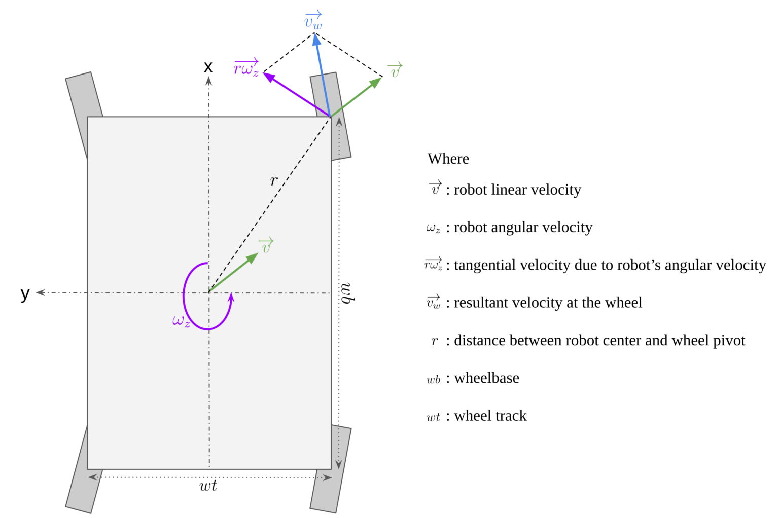
A simple omnidirectional platform is mecanum wheel chassis. But for a FRC player, a swerve chassis is what we need.

Consider only the translation case. Let's simply denote $(x,y)$ for position, $v$ for velocity, $a$ for acceleration, $\theta$ for angle, $\omega$ for angular velocity, $\alpha$ for angular acceleration.

$$\left[\begin{array}{c}\dot{x}\\ \dot{y}\\ \dot{v}\\ \dot{\theta }\\ \dot{\omega }\end{array}\right]=\left[\begin{array}{c}v\cos \theta \\ v\sin \theta \\ a\\ \omega \\ \alpha \end{array}\right]$$

So that, we can use the following equation to update the states in discrete time domian.

$$\{\begin{array}{l}{v}_{k+1}=v_k+a\cdot \mathrm{\Delta }t\\ {\omega }_{k+1}={\omega }_k+\alpha \cdot \mathrm{\Delta }t\\ {\theta }_{k+1}={\theta }_k+\frac{1}{2}({\omega }_k+{\omega }_{k+1})\cdot \mathrm{\Delta }t\\ x_{k+1}=x_k+\frac{1}{2}(v_k\cos {\theta }_k+v_{k+1}\cos {\theta }_{k+1})\cdot \mathrm{\Delta }t\\ y_{k+1}=y_k+\frac{1}{2}(v_k\sin {\theta }_k+v_{k+1}\sin {\theta }_{k+1})\cdot \mathrm{\Delta }t\end{array},u_k=\left[\begin{array}{c}a\\ \alpha \end{array}\right]$$

Objective Function

Denote the number of control points of optimal control is $M$, and ${\overline{u}}_k={\left[\begin{array}{ccc}{u}_k^T& u_{k+1}^T& \cdots u_{k+M-1}^T\end{array}\right]}^T\in {\mathbb{R}}^{2M}$

$$\text{L}oss({\overline{u}}_k)=\sum _{i=0}^{M-1}\left[\begin{array}{rl}& (x_{k+i}-{\hat{x}}_{k+1}{)}^2+\\ & (y_{k+i}-{\hat{y}}_{k+1}{)}^2+\\ & {\omega }_a(a_{k+i-1}-a_{k+i}{)}^2+\\ & {\omega }_{\alpha }({\alpha }_{k+i-1}-{\alpha }_{k+1}{)}^2\end{array}\right]$$$$\begin{array}{rl}\underset{{\overline{u}}_k}{min}& \text{L}oss({\overline{u}}_k)\\ \text{s}.t.& a_{min}\le a_i\le a_{max},& \mathrm{\forall }i\in [k,k+M-1]\\ & {\alpha }_{min}\le {\alpha }_i\le {\alpha }_{max},& \mathrm{\forall }i\in [k,k+M-1]\end{array}$$

The method to solve this objective function is similar to the PHR ALM method mentioned above, except that the terms related to the symmetric cone are removed.

Reference

Image	Link
	https://mathworld.wolfram.com/images/eps-svg/CubicSpline_700.svg
	https://www.tandfonline.com/cms/asset/bc9fed8a-15a8-49ee-96be-ce81ead2a54b/tgis_a_1988088_f0001_b.gif
	https://www.freshconsulting.com/wp-content/uploads/2023/02/image-1536x1022.png